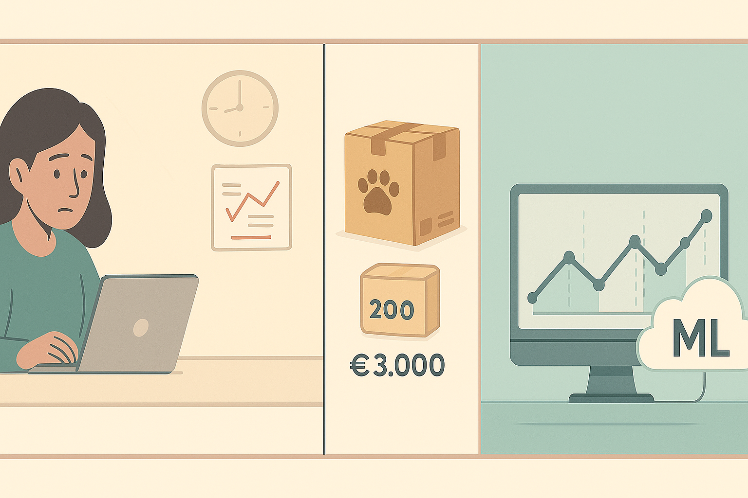
It's 9:00 AM on a Monday and María, owner of an online pet products store, reviews her weekend numbers. Her star product sold out on Friday, losing 47 potential sales. Meanwhile, she has 200 units of a toy that barely moves, immobilizing €3,000 in capital. This situation repeats weekly in thousands of Spanish SMEs.
68% of small retail businesses regularly lose sales due to stockouts, while 34% have overstock problems that affect their cash flow. Demand forecasting with Machine Learning is no longer an exclusive luxury of Amazon or El Corte Inglés: it's within reach of any SME that wants to optimize its inventory.
What is Machine Learning for Demand Forecasting?
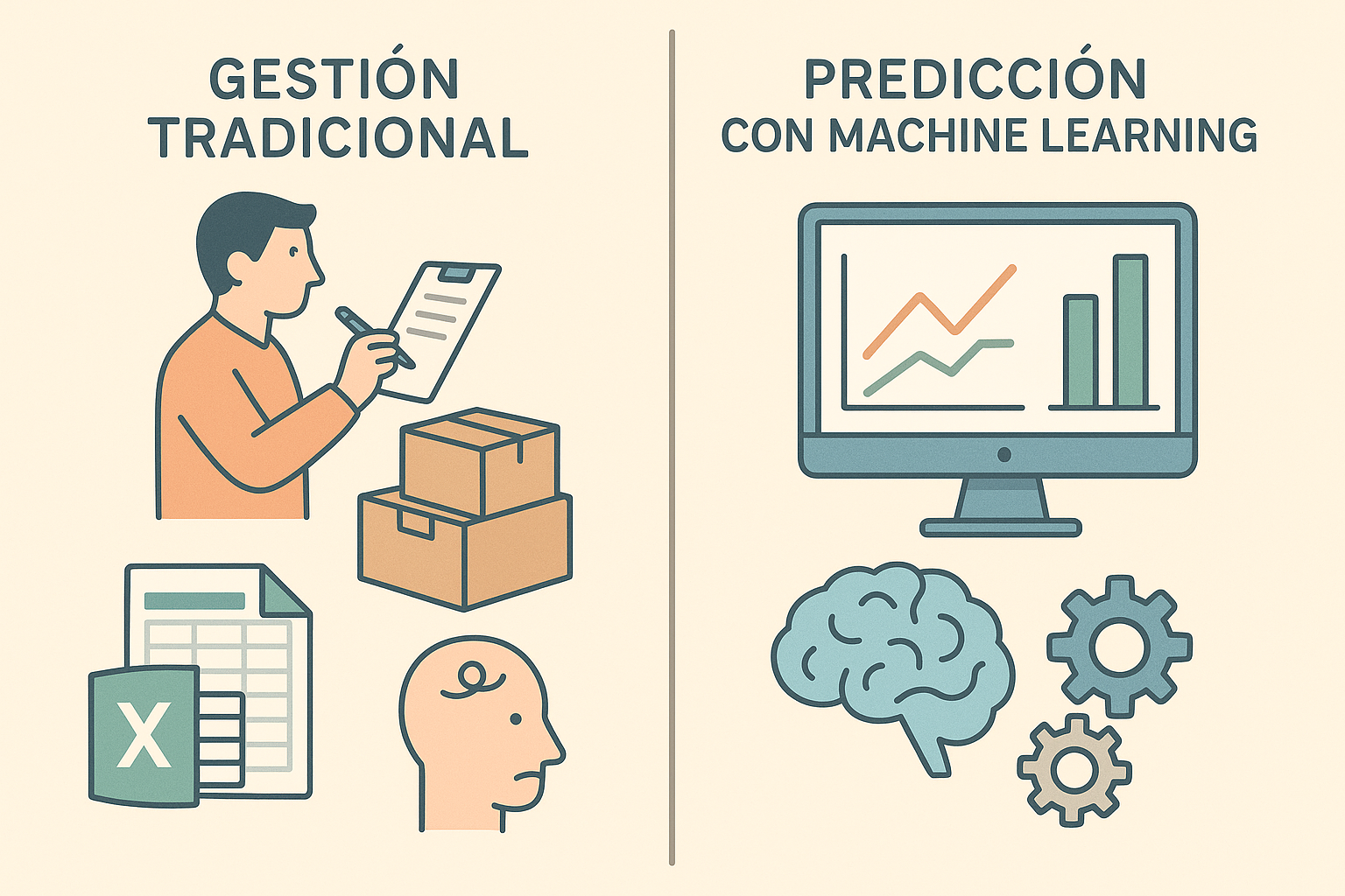
Machine Learning for demand forecasting is a branch of artificial intelligence that analyzes historical sales patterns, seasonality, trends, and external factors to predict how many products will be sold in future periods. Unlike traditional methods based on intuition or simple averages, ML can process thousands of variables simultaneously.
For an SME, this means moving from purchase decisions based on 'feeling' to precise predictions backed by data. The algorithm learns from your sales history, identifies seasonal patterns, detects emerging trends, and automatically adjusts predictions according to special events like promotions or holidays.
The Real Cost of Not Predicting Demand
SMEs that don't use demand forecasting face hidden costs that can represent up to 30% of their potential revenue. These costs manifest in multiple ways and directly affect business profitability and growth.
Stockouts: Lost Sales
- Direct loss of sales when the product is not available
- Customers who migrate to competitors and may not return
- Damage to reputation and customer trust
- Loss of positioning in marketplaces like Amazon or Mercado Libre
- Negative impact on reviews and ratings
Excess Inventory: Immobilized Capital
- Working capital blocked in products that don't move
- Storage and maintenance costs
- Risk of obsolescence, especially in technology and fashion
- Need to liquidate with discounts that erode margins
- Lost opportunity to invest in high-rotation products
According to studies by the Spanish Confederation of Commerce, SMEs lose on average 23% of potential sales due to inventory management problems, equivalent to €47,000 annually for a company with €500,000 in revenue.
Historical Data Needed to Get Started
Effective prediction with Machine Learning requires quality historical data. For SMEs just starting, the good news is that they don't need years of information: with 6-12 months of basic data they can already obtain useful predictions.
Essential Basic Data
| Data Type | Description | Minimum Frequency | Impact on Accuracy |
|---|---|---|---|
| Sales per product | Units sold per SKU | Daily | High |
| Sale dates | Timestamp of each transaction | Daily | High |
| Historical prices | Sale price in each period | Weekly | Medium |
| Stock level | Available inventory by date | Daily | Medium |
| Promotions | Discounts and offers applied | Per event | High |
| Product category | Product classification | Per SKU | Medium |
Advanced Context Data
To significantly improve prediction accuracy, especially in seasonal businesses, it's recommended to include external context data:
- Holiday calendar: Christmas, Black Friday, Mother's Day, etc.
- Weather events: Especially important for clothing, gardening, sports
- Search trends: Google Trends for specific products
- Marketing campaigns: Advertising investment and channels used
- Competitive events: Competitor launches, price changes
- Macroeconomic factors: Consumer confidence indices
Data Preparation for ML
import pandas as pd
import numpy as np
from datetime import datetime, timedelta

def prepare_sales_data(sales_file):
    """
    Prepare sales data for demand forecasting models
    """
    # Load sales data
    df = pd.read_csv(sales_file)

    # Convert date to datetime
    df['date'] = pd.to_datetime(df['date'])

    # Add temporal features
    df['year'] = df['date'].dt.year
    df['month'] = df['date'].dt.month
    df['day_of_week'] = df['date'].dt.dayofweek
    df['day_of_month'] = df['date'].dt.day
    df['week_of_year'] = df['date'].dt.isocalendar().week

    # Identify holidays (example for Spain)
    spanish_holidays = [
        '2024-01-01', '2024-01-06', '2024-04-01', '2024-05-01',
        '2024-08-15', '2024-10-12', '2024-11-01', '2024-12-06',
        '2024-12-08', '2024-12-25'
    ]

    df['is_holiday'] = df['date'].dt.strftime('%Y-%m-%d').isin(spanish_holidays)

    # Detect high demand periods
    df['is_black_friday'] = (
        (df['month'] == 11) &
        (df['day_of_week'] == 4) &
        (df['day_of_month'] >= 22) &
        (df['day_of_month'] <= 28)
    )

    df['is_christmas'] = (
        (df['month'] == 12) &
        (df['day_of_month'] >= 15)
    )

    # Calculate lag features (previous sales)
    for product in df['product_id'].unique():
        mask = df['product_id'] == product
        df.loc[mask, 'sales_lag_7'] = df.loc[mask, 'units_sold'].shift(7)
        df.loc[mask, 'sales_lag_30'] = df.loc[mask, 'units_sold'].shift(30)
        df.loc[mask, 'moving_avg_7'] = df.loc[mask, 'units_sold'].rolling(7).mean()
        df.loc[mask, 'moving_avg_30'] = df.loc[mask, 'units_sold'].rolling(30).mean()

    # Calculate growth trend
    df['trend_7d'] = (df['moving_avg_7'] - df['sales_lag_7']) / df['sales_lag_7']

    # Detect seasonal products
    df['coef_variation'] = df.groupby('product_id')['units_sold'].transform(
        lambda x: x.std() / x.mean() if x.mean() > 0 else 0
    )

    # Mark seasonal products (high variability)
    df['is_seasonal'] = df['coef_variation'] > 0.5

    # Clean null values
    df = df.fillna(0)

    return df

# Usage example
# prepared_data = prepare_sales_data('historical_sales.csv')
# print(f"Prepared data: {prepared_data.shape[0]} records with {prepared_data.shape[1]} features")
Machine Learning Algorithms Explained
For SMEs without deep technical background, it's important to understand that not all ML algorithms are equally complex or appropriate for demand forecasting. We'll start with the most accessible and effective for real-world use cases.
Linear Regression: The Starting Point
Linear regression is the simplest and most understandable algorithm for demand forecasting. It establishes a mathematical relationship between known variables (like historical sales, seasonality, prices) and expected future sales.
- Advantages: Easy to understand, quick to train, interpretable
- Disadvantages: Assumes linear relationships, limited for complex patterns
- Ideal for: Products with stable demand, B2B businesses, initial analysis
- Expected accuracy: 70-85% for products with simple patterns
from sklearn.linear_model import LinearRegression
from sklearn.model_selection import train_test_split
from sklearn.metrics import mean_absolute_error, mean_squared_error
import numpy as np

def simple_regression_model(data):
    """
    Implements a linear regression model for demand forecasting
    """
    # Select relevant features
    features = [
        'day_of_week', 'month', 'is_holiday', 'is_black_friday',
        'sales_lag_7', 'moving_avg_30', 'price'
    ]

    X = data[features]
    y = data['units_sold']

    # Split into training and test
    X_train, X_test, y_train, y_test = train_test_split(
        X, y, test_size=0.2, random_state=42, shuffle=False
    )

    # Train model
    model = LinearRegression()
    model.fit(X_train, y_train)

    # Make predictions
    y_pred = model.predict(X_test)

    # Evaluate performance
    mae = mean_absolute_error(y_test, y_pred)
    rmse = np.sqrt(mean_squared_error(y_test, y_pred))

    # Calculate accuracy as percentage
    mape = np.mean(np.abs((y_test - y_pred) / y_test)) * 100

    print(f"Mean Absolute Error: {mae:.2f} units")
    print(f"Root Mean Square Error: {rmse:.2f} units")
    print(f"Mean Absolute Percentage Error: {mape:.1f}%")
    print(f"Model accuracy: {100-mape:.1f}%")

    # Show feature importance
    importance = pd.DataFrame({
        'feature': features,
        'coefficient': model.coef_,
        'abs_importance': np.abs(model.coef_)
    }).sort_values('abs_importance', ascending=False)

    print("\nFeature importance:")
    print(importance)

    return model, mae, rmse, mape

# Function to predict future sales
def predict_future_demand(model, base_data, future_days=30):
    """
    Predicts demand for the next N days
    """
    # Get the last record as base
    last_record = base_data.iloc[-1].copy()
    predictions = []

    for day in range(1, future_days + 1):
        # Update date
        future_date = last_record['date'] + timedelta(days=day)

        # Update temporal features
        last_record['day_of_week'] = future_date.dayofweek
        last_record['month'] = future_date.month
        last_record['day_of_month'] = future_date.day

        # Prepare data for prediction
        X_future = last_record[[
            'day_of_week', 'month', 'is_holiday', 'is_black_friday',
            'sales_lag_7', 'moving_avg_30', 'price'
        ]].values.reshape(1, -1)

        # Predict
        prediction = model.predict(X_future)[0]
        predictions.append({
            'date': future_date,
            'predicted_demand': max(0, int(prediction))  # Cannot be negative
        })

        # Update lag features for next iteration
        last_record['sales_lag_7'] = prediction

    return pd.DataFrame(predictions)
Random Forest: Power without Complexity
Random Forest is significantly more powerful than linear regression for capturing complex patterns, but maintains ease of use. It's especially effective for products with seasonal behaviors or influenced by multiple factors.
- Advantages: Handles non-linear relationships, resistant to outliers, doesn't require normalization
- Disadvantages: Less interpretable than linear regression, can overfit with little data
- Ideal for: Seasonal products, wide catalogs, e-commerce with frequent promotions
- Expected accuracy: 80-92% for most use cases
Time Series with ARIMA
ARIMA (AutoRegressive Integrated Moving Average) is specifically designed for time series data and is excellent for automatically identifying trends and seasonalities.
- Advantages: Designed for time series, identifies trends automatically
- Disadvantages: Requires stationary data, difficulty with external variables
- Ideal for: Products with clear seasonal patterns, trend analysis
- Expected accuracy: 75-88% for series with stable patterns
Tangible Benefits for Your SME
The benefits of implementing retail machine learning go beyond simply predicting numbers. They translate into concrete operational improvements that directly impact the company's balance sheet.
Stock and Working Capital Optimization
| Metric | Before ML | After ML | Improvement |
|---|---|---|---|
| Average stock level | 45 days | 28 days | -38% |
| Monthly stockouts | 12% | 3% | -75% |
| Immobilized capital | €85,000 | €53,000 | -38% |
| Margin lost to discounts | 8% | 2% | -75% |
| Time in inventory management | 15 hrs/week | 4 hrs/week | -73% |
Impact on Sales and Customer Satisfaction
- 15-25% increase in sales due to better availability of popular products
- Improvement in customer experience by reducing cancellations due to stockouts
- Increase in average order value by optimizing product mix
- 60% reduction in response time to demand changes
- Improvement in marketplace metrics (Amazon, eBay) due to better availability
McKinsey & Company study (2023) shows that SMEs implementing demand forecasting with ML see an average 19% increase in sales and 32% reduction in inventory costs during the first year.
Accessible Tools for SMEs
The democratization of Machine Learning has brought tools specifically designed for SMEs that don't require deep technical expertise or massive infrastructure investments.
No-Code/Low-Code Solutions
| Tool | Type | Monthly Price | Specialty |
|---|---|---|---|
| Inventory Planner | SaaS | €249-599 | Shopify, WooCommerce |
| Lokad | SaaS | €500-2000 | E-commerce, retail |
| DataRobot | ML Platform | €1000-3000 | Automated ML |
| H2O.ai | AutoML | €300-800 | Automated prediction |
| Amazon Forecast | Cloud API | €0.60/1000 pred | AWS integrated |
| Google Vertex AI | Cloud ML | €0.40/1000 pred | Google Cloud |
Open Source Tools
For SMEs with internal technical resources or very limited budgets, there are excellent open source options that can be implemented internally:
- Prophet (Facebook): Specialized in time series with seasonality
- Scikit-learn: Complete ML library for Python
- Statsmodels: Advanced statistical and econometric analysis
- TensorFlow: For more sophisticated deep learning models
- R + Forecast package: Excellent for traditional statistical analysis
Integration with Existing Platforms
# Example integration with Shopify to get sales data
import shopify
import pandas as pd
from datetime import datetime, timedelta

def extract_shopify_data(api_key, password, shop_name, historical_days=365):
    """
    Extract sales data from Shopify for ML training
    """
    # Configure connection
    shopify.ShopifyResource.set_site(f"https://{api_key}:{password}@{shop_name}.myshopify.com/admin")

    # Start date
    start_date = datetime.now() - timedelta(days=historical_days)

    # Get orders
    orders = shopify.Order.find(
        status='any',
        created_at_min=start_date.isoformat(),
        limit=250
    )

    sales_data = []

    for order in orders:
        for item in order.line_items:
            sales_data.append({
                'date': pd.to_datetime(order.created_at).date(),
                'product_id': item.product_id,
                'variant_id': item.variant_id,
                'sku': item.sku,
                'product_name': item.name,
                'units_sold': item.quantity,
                'unit_price': float(item.price),
                'total_sales': float(item.price) * item.quantity,
                'discount': float(getattr(item, 'total_discount', 0))
            })

    df = pd.DataFrame(sales_data)

    # Aggregate by day and product
    df_aggregated = df.groupby(['date', 'product_id', 'sku']).agg({
        'units_sold': 'sum',
        'unit_price': 'mean',
        'total_sales': 'sum',
        'product_name': 'first'
    }).reset_index()

    return df_aggregated

# Example integration with WooCommerce
from woocommerce import API

def extract_woocommerce_data(url, consumer_key, consumer_secret, historical_days=365):
    """
    Extract sales data from WooCommerce
    """
    wcapi = API(
        url=url,
        consumer_key=consumer_key,
        consumer_secret=consumer_secret,
        version="wc/v3",
        timeout=30
    )

    # Start date
    start_date = datetime.now() - timedelta(days=historical_days)

    # Get orders
    orders = wcapi.get("orders", params={
        "after": start_date.isoformat(),
        "status": "completed",
        "per_page": 100
    })

    sales_data = []

    for order in orders.json():
        for item in order['line_items']:
            sales_data.append({
                'date': pd.to_datetime(order['date_created']).date(),
                'product_id': item['product_id'],
                'sku': item['sku'],
                'product_name': item['name'],
                'units_sold': item['quantity'],
                'unit_price': float(item['price']),
                'total_sales': float(item['total'])
            })

    return pd.DataFrame(sales_data)

# Unified function for multiple platforms
def get_sales_data(platform, **kwargs):
    """
    Unified function to extract data from different platforms
    """
    if platform == 'shopify':
        return extract_shopify_data(**kwargs)
    elif platform == 'woocommerce':
        return extract_woocommerce_data(**kwargs)
    else:
        raise ValueError(f"Platform {platform} not supported")
Step-by-Step Implementation for SMEs
The key to success in implementing AI inventory management is following a gradual approach that minimizes risks while building confidence in the system.
Phase 1: Data Audit (Week 1-2)
- Inventory of existing data sources (e-commerce platform, ERP, spreadsheets)
- Quality assessment: completeness, consistency, update frequency
- Identification of critical missing data and plan to obtain it
- Selection of 5-10 representative products for pilot project
- Configuration of automatic data collection system
Phase 2: Pilot Model Development (Week 3-6)
- Cleaning and preparation of historical data (minimum 6 months)
- Implementation of basic model (linear regression or Random Forest)
- Training with 80% of data, validation with remaining 20%
- Backtesting: compare predictions with actual sales from last month
- Parameter adjustment to optimize accuracy
Phase 3: Production Testing (Week 7-10)
- Implementation on selected pilot products
- Side-by-side comparison: traditional management vs ML predictions
- Daily monitoring of accuracy and inventory adjustments
- Documentation of results and lessons learned
- Calculation of initial ROI and improvement metrics
Phase 4: Scaling (Week 11+)
- Gradual expansion to entire product catalog
- Automation of purchase processes based on predictions
- Integration with suppliers to optimize lead times
- Implementation of automatic alerts and dashboards
- Team training in system interpretation and use
Success Metrics and KPIs
Defining clear metrics from the start is crucial to evaluate the real impact of demand forecasting software on your business. These metrics should be easy to measure and directly related to business results.
Model Accuracy Metrics
| Metric | Description | Target | Frequency |
|---|---|---|---|
| MAPE | Mean absolute percentage error | <15% | Weekly |
| Accuracy by category | Accuracy by product type | >80% | Monthly |
| Prediction bias | Tendency to over/underestimate | ±5% | Weekly |
| Forecast vs Actual | Visual comparison of trends | Tracking | Daily |
Business Impact Metrics
| KPI | Baseline | 6-month Target | 12-month Target |
|---|---|---|---|
| Stockout rate | 12% | 6% | 3% |
| Inventory turnover | 6.2x/year | 8.5x/year | 10x/year |
| Average stock days | 45 days | 32 days | 25 days |
| Gross margin | 32% | 35% | 38% |
| Customer satisfaction | 4.2/5 | 4.5/5 | 4.7/5 |
import pandas as pd
import matplotlib.pyplot as plt
import seaborn as sns
from datetime import datetime, timedelta

class MLMonitoring:
    def __init__(self):
        self.historical_metrics = []

    def calculate_mape(self, y_real, y_predicted):
        """
        Calculate Mean Absolute Percentage Error
        """
        return np.mean(np.abs((y_real - y_predicted) / y_real)) * 100

    def calculate_bias(self, y_real, y_predicted):
        """
        Calculate prediction bias (tendency to over/underestimate)
        """
        return np.mean((y_predicted - y_real) / y_real) * 100

    def evaluate_daily_model(self, date, predictions, actual_sales):
        """
        Evaluate model performance for a specific day
        """
        mape = self.calculate_mape(actual_sales, predictions)
        bias = self.calculate_bias(actual_sales, predictions)

        # Calculate additional metrics
        mae = np.mean(np.abs(actual_sales - predictions))
        rmse = np.sqrt(np.mean((actual_sales - predictions)**2))

        metrics = {
            'date': date,
            'mape': mape,
            'bias': bias,
            'mae': mae,
            'rmse': rmse,
            'accuracy': max(0, 100 - mape),
            'num_products': len(predictions)
        }

        self.historical_metrics.append(metrics)
        return metrics

    def generate_weekly_report(self):
        """
        Generate weekly performance report
        """
        if len(self.historical_metrics) < 7:
            print("Insufficient data for weekly report")
            return

        # Get last 7 days
        df_metrics = pd.DataFrame(self.historical_metrics[-7:])

        # Calculate weekly statistics
        report = {
            'average_mape': df_metrics['mape'].mean(),
            'median_mape': df_metrics['mape'].median(),
            'average_bias': df_metrics['bias'].mean(),
            'average_accuracy': df_metrics['accuracy'].mean(),
            'days_meeting_target': (df_metrics['mape'] < 15).sum(),
            'improvement_trend': df_metrics['mape'].iloc[-3:].mean() < df_metrics['mape'].iloc[:3].mean()
        }

        # Generate alert if necessary
        if report['average_mape'] > 20:
            print("⚠️ ALERT: Accuracy below target")
            print(f"Average MAPE: {report['average_mape']:.1f}% (target: <15%)")

        return report

    def metrics_dashboard(self):
        """
        Create visual metrics dashboard
        """
        df = pd.DataFrame(self.historical_metrics)

        fig, axes = plt.subplots(2, 2, figsize=(15, 10))

        # MAPE over time
        axes[0,0].plot(df['date'], df['mape'])
        axes[0,0].axhline(y=15, color='r', linestyle='--', label='Target')
        axes[0,0].set_title('MAPE Evolution')
        axes[0,0].set_ylabel('MAPE (%)')
        axes[0,0].legend()

        # Bias over time
        axes[0,1].plot(df['date'], df['bias'])
        axes[0,1].axhline(y=0, color='g', linestyle='-', alpha=0.3)
        axes[0,1].axhline(y=5, color='r', linestyle='--', label='Limit')
        axes[0,1].axhline(y=-5, color='r', linestyle='--')
        axes[0,1].set_title('Prediction Bias')
        axes[0,1].set_ylabel('Bias (%)')
        axes[0,1].legend()

        # Error distribution
        axes[1,0].hist(df['mape'], bins=20, alpha=0.7)
        axes[1,0].axvline(x=15, color='r', linestyle='--', label='Target')
        axes[1,0].set_title('Error Distribution')
        axes[1,0].set_xlabel('MAPE (%)')
        axes[1,0].legend()

        # Accuracy by day of week
        df['day_of_week'] = pd.to_datetime(df['date']).dt.day_name()
        accuracy_by_day = df.groupby('day_of_week')['accuracy'].mean()
        axes[1,1].bar(accuracy_by_day.index, accuracy_by_day.values)
        axes[1,1].set_title('Accuracy by Day of Week')
        axes[1,1].set_ylabel('Accuracy (%)')
        axes[1,1].tick_params(axis='x', rotation=45)

        plt.tight_layout()
        plt.show()

        return fig

# Usage example
monitor = MLMonitoring()

# Simulate daily evaluation
for i in range(30):
    date = datetime.now() - timedelta(days=30-i)
    # Simulate predictions vs actual sales
    predictions = np.random.normal(100, 20, 50)
    actual_sales = predictions + np.random.normal(0, 15, 50)

    metrics = monitor.evaluate_daily_model(date, predictions, actual_sales)

report = monitor.generate_weekly_report()
print(f"Average accuracy last week: {report['average_accuracy']:.1f}%")